Create team comparisons

Part 1: Download reports

If you are not familiar with the locations of these reports, follow these links:

• Site history
• Users
• Groups
• User2group

Part 2: Combine reports into a single CSV

Please review this document on how to merge multiple reports within Excel.

1. Merge the four reports into a single Excel workbook.
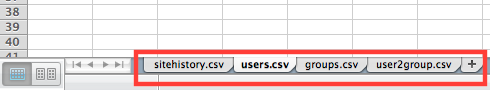
2. Rename the site history report to a more concise sitehistory.csv (concise names will be easier to manage when reviewing functions).
3. Once you've merged your reports into a single workbook, your tab structure should look like the following screenshot.

Part 3: Label your lists and data tables (optional)

This is not a necessary step, but it will help to define more intuitive functions going forward.

Label the following lists:

• SITEHISTORY_TYPE 
• SITEHISTORY_USERID 
• GROUPS_GROUPID 
• USER2GROUP_GROUPID 
• USER2GROUP_USERID 
• USERS_USERID
• USERS_USERNAME

To label data tables, highlight the entire data table and label it as you would a list. Label the following data tables:

• GROUPS
• USER2GROUP

Part 4: Combine all sheets into one group based sheet

Use VLOOKUP() and Data Validation to merge data from the four reports into a single sheet, titled Group Selector:

1. Create a new sheet and title it "Group Selector".
2. From the sitehistory.csv sheet, copy column E (USER ID) and paste into column A within the Group Selector sheet.

3. In cell B1, enter the header IN GROUP.

Part 5: Create a group selector drop-down

To enable the easy designation of the desired group, we will create a GROUP ID drop-down list.

1. Create a new sheet and title it Leaderboard.
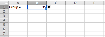
2. Title cell A1 "Group =".
3. Click on cell B1.
4. Select Validate from the Data menu.

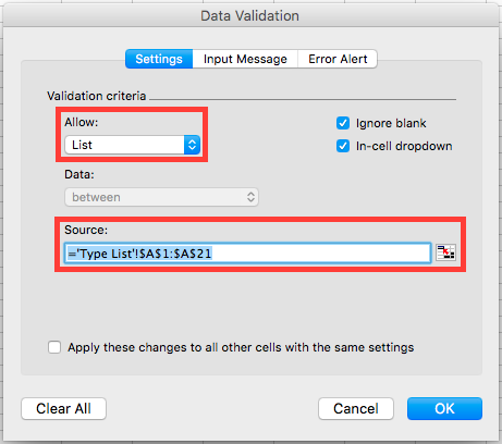
3. Within the Data Validation pop up window:

• Select List from the Allow options drop-down list.
• Under the Source section, select the full list of GROUP IDs from the groups.csv sheet.

4. You will now see the GROUP ID drop-down appear in cell B1.

5. To pull the GROUP NAME for the specified GROUP ID, click on cell C1, and add the following function:

=VLOOKUP(B1,GROUPS,2,FALSE())

6. When a GROUP ID is selected, the associated GROUP NAME will also populate.

Part 6: Track users within your desired group

1. From the groups.csv sheet, find the GROUP ID associated with your desired group. In this example, for GROUP NAME, Engineering, the associated GROUP ID is 9.

2. From the Leaderboard sheet select GROUP ID 9 from the GROUP ID drop-down. GROUP NAME Engineeringalso populates.

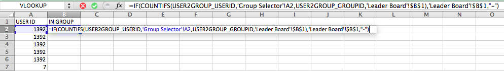
3. From the Group Selector sheet, enter the following formula into cell B.

=IF(COUNTIFS(USER2GROUP_USERID,'Group Selector'!A2,USER2GROUP_GROUPID,'Leaderboard'!$B$1),'Leaderboard'!$B$1,"-")

4. To populate the entire IN GROUP column, highlight B2, and drag it down to the bottom of the list (or double click the square at the bottom right-hand side of the highlighted selection.

5. Label the IN GROUP list GROUPSELECTOR_INGROUP using the process described in Part 3.

COUNTIFS(criteria_range1, criteria1, criteria_range2, criteria2,...)

=IF(COUNTIFS(USER2GROUP_USERID,'Group Selector'!A2,USER2GROUP_GROUPID,'Leaderboard'!$B$1),'Leaderboard'!$B$1,"-")

IF(logical_test, [value_if_true], [value_if_false])

=IF(COUNTIFS(USER2GROUP_USERID,'Group Selector'!A2,USER2GROUP_GROUPID,'Leaderboard'!$B$1),'Leaderboard'!$B$1,"-")

Part 7: Create a list of all activity types

Now that you are able to track users by group, you can take the necessary steps to track user activity by a given type.  In this part, we will create a list of all possible TYPE options.

1. Create a new sheet and title it "Type List."
2. From the sitehistory.csv sheet, copy column D (TYPE) and paste into column A within the Type List sheet.
3. With the list highlighted, choose Remove Duplicates from the Data menu.

4. The resulting list includes the full TYPE list.
5. Label the TYPE list, TYPE_LIST, using the process described in Part 3.

Part 8: Track user activity

Now that we can access a full TYPE list, let's track user activity against a given TYPE: 

1. Create a new sheet, and title it Track User Activity.
2. Copy the entire User ID list from the users.csv sheet and past it to column B of the Track User Activity sheet.

In column C , we are going to track users within the specified group against a given activity type.  To do so:

3. Title cell C1 "Type =".
4. Click on cell D1.
5. Choose Validate from the Data menu.

6. Within the Data Validation pop up window:

• Select List from the Allow options drop-down list.
• Under the Source section, select the full list of types from the Type List sheet.

7. You will now see the Type drop-down appear in cell D1.

8. From the Track User Activity sheet, enter the following formula into cell C2: 

=COUNTIFS(SITEHISTORY_USERID,'Track User Activity'!B2,GROUPSELECTOR_INGROUP,'Leaderboard'!$B$1,SITEHISTORY_TYPE,'Track User Activity'!$D$1)

9. To populate the entire Type = column, highlight C2, and drag it down to the bottom of the list (or double click the square at the bottom right-hand side of the highlighted selection.

Part 9: Rank your top 10 users

Now that we can easily track users within a group by the desired activity type, let's start to create a leaderboard for the top 10 users. First, we will need to rank users within a specified group by the number of times they have completed a specified activity type:

1. Within the Track User Activity sheet, title cell A1 "RANK."
2. Enter the following formula into cell A2:  

=IF(C2=0,0,RANK(C2,$C$2:$C$1925)+COUNTIF($C$2:C2,C2)-1)

3. To populate the entire RANK column, highlight A2, and drag it down to the bottom of the list (or double click the square at the bottom right-hand side of the highlighted selection.

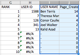
Part 10: Build a table for your top 10 users

1. Give the following titles to the following cells:
   1. G1: "RANK"
   2. H1: "USER ID"
   3. I1: "USER NAME"
2. Enter the following formula into cell J1:

   =D1

   Column J will list the number of times the specified activity type is completed for a given user.  The title of that column will be the activity type.
    
3. Under the RANK header, number the fields G2 through G11 1 through 10.
4. In cell H2, under the header USER ID, add the following:

   =VLOOKUP(G2,$A$1:$C$1925,2,FALSE())
   

   This function returns the user ID associated with the referenced rank.
    
5. In cell I2, under the header USER NAME, add the following:

   =IFERROR(VLOOKUP(H2,users.csv!$A$1:$I$1925,4,FALSE()),"-")
   

   This function returns the user name associated with the referenced user ID.
    
6. In cell J2, under the activity type, add the following:

   =IFERROR(VLOOKUP(H2,$B$2:$C$1925,2,FALSE()),0)
   

   This function returns the total activities of the specified type associated with the referenced user ID.
    
7. To populate the entire top 10 list, highlight H2-J2 and drag them down to the bottom of the list (or double click the square at the bottom right-hand side of the highlighted selection.

Part 11: Create a chart for your leaderboard                                       

Now that you've created your top 10 list, the final step is to add a chart to your Leaderboard sheet.

1. Select the User Name and activity type columns within the top 10 list of your of the Track User Activity sheet.

2. Choose a chart type from the Charts menu (in this example I've selected the Column option).

3. A chart is now created for your leaderboard.

4. Cut and paste this chart into your leaderboard.

Part 12: Add new charts to your leaderboard

1. Right-click the Track User Activity sheet tab.
2. Select Move or Copy.
3. Check the box labeled, Create a copy.
4. Click OK.
5. Click on the Type drop-down (in cell D1) to select an alternative activity type.
6. Follow the process of creating a leaderboard in Part 11.